Logistic Regression
Classification
In a classification problem a classifier (a piece of software) maps the inputs to a small and discrete set of outputs. For example, classifying incoming emails into (i) the spam folder, or (ii) the inbox folder.
In a Binary classification problem there are only two possible outputs. We can label these groups as 1 (positive class) and 0 (negative class), $y\in \{0,1\}$. For instance, a binary classification problems can be
- Email: Spam/Not Spam?
- Online Transactions: Fradulent(yes/No)?
- Tumor: Malignant/Benign?
Since classification is not a linear function, using linear regression to solve a classification can be a bad choice.
Hypothesis representation
We are going to use logistic regression to solve calssification problems. Logistic regression hypothesis accepts arbitrary inputs and bounds the output between zero and one, $0 \leq y \leq 1$.
The logistic regression hypothesis function is constructed by feeding a sigmoid (or logistic) function a linear model. A sigmoid function ($g(z)=\frac{1}{1+e^-z}$) has the following shape

By replacing $z$ with a linear (or polynomial) function $\theta_0 + \theta_1 x_1 + \dots$ (written in linear algebra notation as $\theta^Tx$) we construct the logistic regression hypothesis function, \begin{equation} h_{\theta}(x) = \frac{1}{1+e^{-\theta^Tx}} \end{equation}
As it can bee seen from the figure and the function form above our new hypothesis takes any number of features and any input values and bounds the output between $0$ and $1$.
To turn this hypothesis function into a binary classifier we need to set a boundary and map some of the output interval to $1$ and the rest to 0. Choosing 0.5 as the boundary result in
- any positive input will be mapped to the output $1$ (positive class),
- any negative input will be mapped to the output $0$ (negrative class), and $h_{\theta}(0)$ draws the decision boundary and separates the area where $y=0$ and where $y=1$. The decision boundary itself can considered as part of the area where $y=0$ or $y=1$, here we choose to make it belong to the area where $y=1$.
Cost Function
The squared error cost function, used with linear regression, results in many local minimum when applied to logistic regression. This prevents gradient descent from finding the global minimum of the cost function. Therefore, we will choose the following cost function which can be shown using maximum likelyhood theory from that it is a convex function--a bow function with a single (global) minimum.
\begin{equation} J(\theta) = -\frac{1}{m} \sum_{i=1}^m[- y^{(i)} \log(h_{\theta}(x^{(i)})) + (1 - y^{(i)}) \log(1- h_{\theta}(x^{(i)}))] \end{equation}
The intuition behind choosing this cost function. Since the output $y$ is either $1$ or $0$ this cost function will be in one of the following two cases:
- case 1: where $y=0$
\begin{equation} J(\theta) = -\frac{1}{m} \sum_{i=1}^m \log(1-h_{\theta}(x^{(i)})) \end{equation}

As we can see from the figure above, when $h_{\theta}(x)$ output $\approx 0$, the error $\approx 0$ also, and when the prediction of $h_{\theta}(x)$ approaches $1$ the error approaches $\infty$
- case 2: where $y=1$
\begin{equation} J(\theta) = -\frac{1}{m} \sum_{i=1}^m \log(h_{\theta}(x^{(i)})) \end{equation}
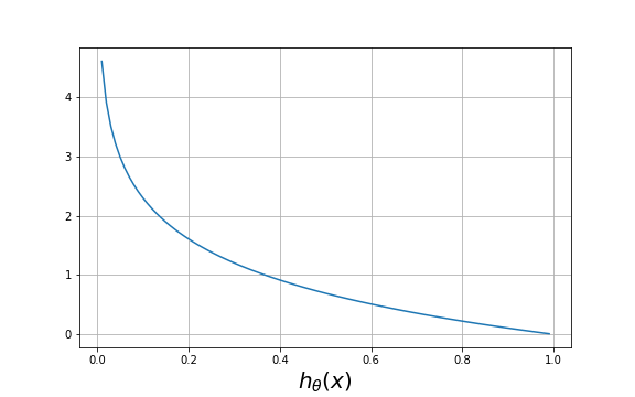
Using analogous arguement we can see that, in case 2, when $h_{\theta}(x)$ output $\approx 1$, the error $\approx 0$ and when $h_{\theta}(x)$ output $\approx 0$, the error $\approx \infty$
Gradient Descent
The Gradient Descent algorithm is
repeat:{ \begin{equation*} \theta_j = \theta_j - \alpha \frac{\partial}{\partial \theta_j} J(\theta) \end{equation*} }.
We can work out the derivative$^1$</sup> using Calculus to get:
repeat:{ \begin{equation*} \theta_j = \theta_j - \frac{\alpha}{m} \sum^m_{i=1}(h_{\theta}(x^{(i)}) - y^{(i)} )x^{(i)}_j \end{equation*} }.
A vectorized implementation of Gradient Descent is:
\begin{equation} \theta=\theta - \frac{\alpha}{m}X^T(g(X\theta) - \overrightarrow{y}) \end{equation}
Logistic Regression for Multi-class classification problem
Some examples of multi-class classification problems include
- Email tagging: tag incoming emailt with labels like 'friends', 'work', 'hobby'.
- Classifying patients with stuffy nose to fine, cold, and flu.
Using the One-vs-all method we can turn a multi-class classification prblem into a set of binary classification problems. Let us consider the email tagging problem. We need to find, using the same procedure for the binary classification problems, three hypotheses (i) one to classify friends vs the rest, (ii) one to classify work vs the rest, and (iii) the last one to classify hobby vs the rest. Any testing input is fed to the three classifiers (hypotheses). The hypothesis that produces the highest output value (as the output of a logistic regression funciton is bounded between 1 and 0) classify the input to its group.
Regularization
Overfitting refers to the problem of generating too complex hypothesis funciton that fits the training data very well, but it does not generalize for new testing data becuase the hypothesis line is very wavy.
TODO use figures to explain
This terminology is applied to both linear and logistic regression. There are two main options to address the issue of overfitting problem:
1) Reduce the number of features:
- Manually select which features to keep.
- Use a model selection algorithm (studied later in the course).
2) Regularization
- Keep all the features, but reduce the magnitude of parameters $\theta_j$.
- Small values of $\theta$ leads to simpler hypothesis which is, in turn, less prone to overfitting.
Regularization works well when we have a lot of slightly useful features.
### Regularized cost function \begin{equation} J(\theta) = \frac{1}{2m} \bigg[\sum_{i=1}^m cost(h_{\theta}(x)-y) + \lambda \sum_{j=1}^n\theta^2_j \bigg] \end{equation} where $cost(h_{\theta}(x)-y)$ can be the part of cost function of linear regression or logistic regression. $\lambda$ is the regularization parameter that controls $\theta$ adaptation.
Advanced Optimization Algorithms
In this section, we show how to use more advanced optimization algorithms like Conjugate gradient, BFGS, and L-BFGS. Octave( or Matlab) provides well developed implementations of these algorithms. These algorithms requires a function that compute the cost function and its partial derivatives. Consider the following example to see how to apply these algorithms.
Example:
Minimize the following cost function $J(\theta)=(\theta_1-5)^2 + (\theta_2-5)^2 $ over $\theta=\begin{bmatrix} \theta_1 \\ \theta_2 \end{bmatrix}$, ($\displaystyle \min_{\theta} J(\theta)$).
To use the advanced optimization algorithms we need to follow the following procedures:
1) write a function that takes $\theta$ and returns the value of the cost function and its partial derivatives at the given $\theta$.
function [Jval, gradient] =  costFunction(theta)
    Jval =  (theta(1) - 5)^2 + (theta(2) -5)^2;
    gradient = zeros(2,1);
    gradient(1) = 2 * (theta(1) - 5);
    gradient(2) = 2 * (theta(2) - 5);
2) Set the maximum number of iterations, the initial $\theta$ values and enable the gradient optimization.
options = optimset('GradObj', 'on', 'MaxIter', '100');
initialTheta = zeros(2,1)
3) Call fminunc (stands for function minimization unconstained). @costFunction is a poiner to the costFunction() function.
[optTheta, functionVal, exitFlag]=fminunc(@costFunction, initialTheta, options);
## Plotting the sigmoid function
import math as m
import matplotlib.pyplot as plt
import numpy as np

%matplotlib inline

y=[]
x=np.arange(-10,10,0.2)
for i in x:
    y.append(1/(1+m.exp(-i)))

plt.figure(figsize=(8,3))
plt.plot(x,y)
plt.grid()
plt.savefig('sigmoid.png')

## Plotting the log functions
import math as m
import matplotlib.pyplot as plt
import numpy as np

%matplotlib inline

y=[]
x=np.arange(0.01,1,0.01)
for i in x:
    y.append(-m.log(i))

plt.figure(figsize=(8,5))
plt.plot(x,y)
plt.grid()
plt.xlabel(r'$h_{\theta}(x)$', fontsize=20)
plt.savefig('minusLog.png')

## Plotting the log functions
import math as m
import matplotlib.pyplot as plt
import numpy as np

%matplotlib inline

y=[]
x=np.arange(0,1,0.01)
for i in x:
    y.append(-m.log(1-i))

plt.figure(figsize=(8,5))
plt.plot(x,y)
plt.grid()
plt.xlabel(r'$h_{\theta}(x)$', fontsize=20)
plt.savefig('oneMinusLog.png')
